CS205 Final Project: Teleporting Parallel MCMC
Laith Alhussein, Nathaniel Burbank, Shawn Pan, Andrew Ross, and Rohan Thavarajah
Introduction
Many of the biggest science applications running today – from climate models [1] to economic forecasting [2] to experimental physics [3] – are probabilistic simulations. Because the models involved are often too complex to integrate analytically, these models generally rely on Monte Carlo methods (basically, drawing lots of samples and taking averages) to make predictions. But even sampling from these simulations can be challenging. To do big science, practitioners must not only contend with increasing data size but also increasing problem complexity.
A specific complexity we are concerned with here (related to the familiar idea of non-convexity) is multimodality. When a probabilistic simulation is multimodal, there isn't a single cluster of likely configurations centered around a characteristic average. Instead, there are multiple such clusters distributed far away from each other in the model's parameter space. One example where this occurs is topic modeling [6], and also in the problem of localizing sensors based on noisy measurements of inter-sensor distance – which is commonly used as a benchmark for multimodal sampling techniques [4], [5].
In this project, we will consider how parallelism can help us deal with problems of big statistical complexity that arise in such applications. We will also introduce a novel method for efficiently sampling from multimodal distributions, analyze its scaling properties, and present our implementation using state-of-the-art parallel computing technologies.
Background
Markov-Chain Monte Carlo
MCMC is a local method for sampling from distributions \(s(x)\). One of its simplest forms is the Metropolis-Hastings algorithm, which works as follows. Assuming you begin at a point \(x_1\), you then propose a point \(x_2\) by sampling from a symmetric proposal distribution \(p(x)\). You then either move there or stay put, and add your current location to the sample chain. The important point is that the ratio of probability of transitioning from \(x_1\) to \(x_2\) and back again must equal the ratio of the target densities \(s(x_1)\) and \(s(x_2)\). If this condition (called "detailed balance") holds, then the sample chain will converge to the true distribution.
Pseudocode for this algorithm is:
and we can write out detailed balance as follows:
Where we relied on using a symmetric proposal distribution \(p(x)\), though there are ways of using non-symmetric proposals.
Regardless of whether a symmetric of non-symmetric proposal distribution is used, MCMC, as a local method, suffers with multimodality (or in general any non-convex density \(s(x)\)), as its local stepping can get stuck in local modes:
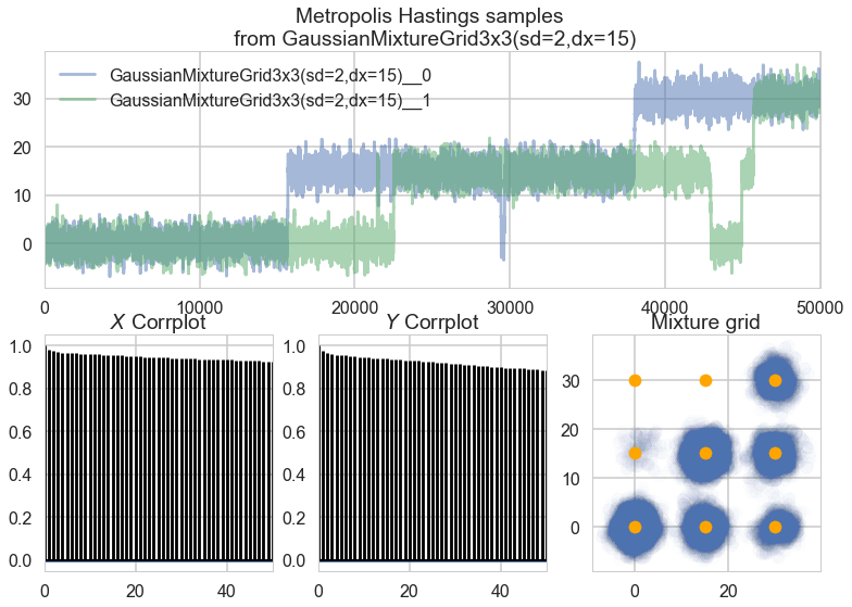
The samples above are from a Metropolis-Hastings sampler, which is a relatively simple MCMC technique. Note that even after removing the first 10% of samples from the chain and further thinning the chain by a factor of 10, there are still very high levels of autocorrelation and the distribution of samples does not reach all of the actual modes. However, even Hamiltonian Monte Carlo, the state of the art, gets stuck in similar ways:
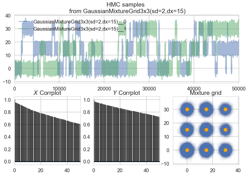
The crux of the problem is that for MCMC to converge, the underlying distribution must be ergodic. Ergodicity is a complex concept but it intuitively corresponds to reachability; every place in the distribution must be reachable from any other via entirely local movements. A mixture of Gaussians like the one from which we sample above technically is ergodic, because the density is never truly 0 anywhere. However, it is only barely ergodic. When our distribution is not ergodic or not ergodic enough, our MCMC samples will be inherently biased.
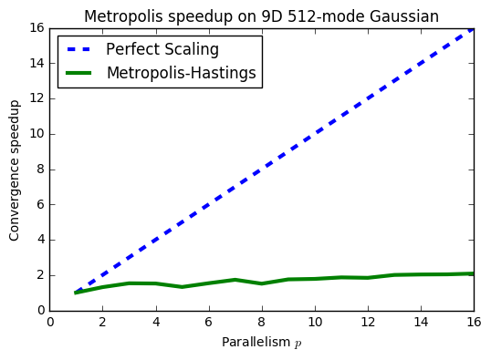
Because of this inherent bias, MCMC can take impractically many iterations to converge, and furthermore, the way its convergence speeds up when combining results from multiple parallel chains is not ideal:
However, MCMC's advantage is that it scales well with dimensions in terms of generating lots of samples (even if they are biased). So while MCMC may take a long time to converge, when it does finally converge, you'll have a lot of samples.
Rejection Sampling
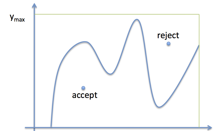
Rejection sampling is at the opposite end of the spectrum from Metropolis-Hastings, though it is also quite simple to describe. In rejection sampling, you essentially draw a giant box enclosing your distribution \(s\):
With psuedocode:
For distributions with infinite support, you can use an encapsulating Gaussian or other analytically samplable distribution in place of a box, or you can approximate one. In any case, you pick a random location within your enclosing distribution, then check to see if it falls underneath \(s\) at that location. If so, you accept it, but otherwise, you reject it. Unlike in MCMC, you discard the rejected samples, and the method is completely global; samples are exactly from \(s\) and entirely uncorrelated with each other (iid).
These properties make rejection sampling quite robust to multimodality. Even with 512 fairly disconnected modes, we see a much better speedup in convergence when combining samples from multiple rejection samplers:

Furthermore, although MCMC is kind of an inherently sequential algorithm since we must build a chain from location to location, rejection sampling can be parallelized at every level (both across nodes using MPI and within nodes using OpenMP).
However, although rejection sampling can handle multimodality, it can't handle multidimensionality. The fraction of samples we accept falls exponentially as the number of dimensions is increased (and the underlying distribution becomes ever more sparse.) This relationship is illustrated by this Gaussian mixture example:
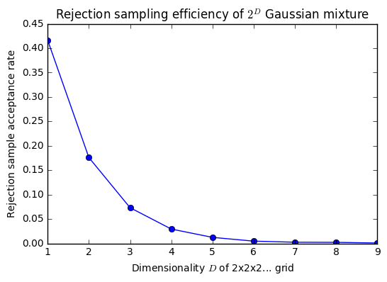
From this analysis, we can consider rejection sampling and MCMC as two different extremes of point-based sampling (and if we use a giant, \(s\)-enclosing proposal distribution for MCMC, they become almost equivalent). But they have exactly the opposite strengths and weaknesses: MCMC handles dimensionality well but not multimodality; rejection sampling handles multimodality well but dimensionality.
Teleporting Hybrid
Our main intuition is to simply linearly interpolate between rejection sampling and MCMC. There is related work ([4], [5]) which attempts to (literally) bridge some of the gaps in MCMC, but to our knowledge, our particular method is novel – though perhaps only because rejection sampling is tricky to set up and becomes inefficient so quickly.
Nevertheless, in our method, during each Metropolis-Hastings step, we either sample from our proposal distribution with probability \(1-\epsilon\) (in which case we accept or reject using the normal MH acceptance probability) or we “teleport” to a new location obtained by rejection sampling with probability \(\epsilon\). Psuedocode is as follows:
In practice, we also return an array of the attempt indexes at which we accepted each sample in order to measure convergence at any iteration.
It is straightforward to show that this scheme, expressed within the framework of traditional Metropolis-Hastings, still satisfies the detailed balance criteria:
Note also that setting \(\epsilon=0\) is exactly Metropolis-Hastings, while \(\epsilon=1\) is exactly rejection sampling; we are linearly interpolating between the two methods.
What we would like to investigate is whether, by choosing an intermediate value for \(\epsilon\), we can obtain samples that allow us to reach convergence more quickly with better parallel scaling.
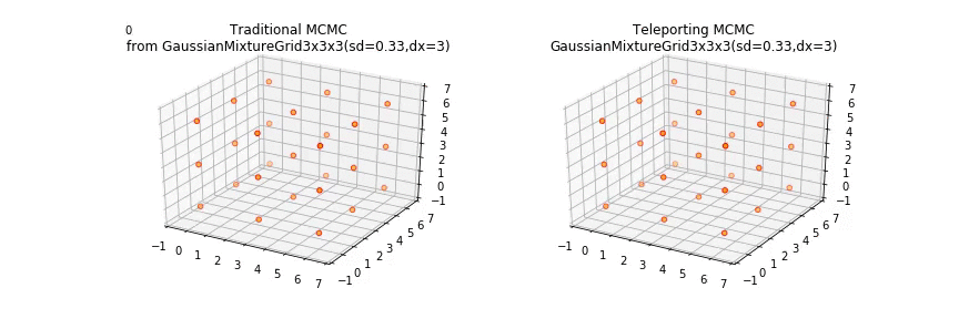
We've animated the difference between \(\epsilon=0\) and \(\epsilon=.0334\) here:
Implementation
Hybrid Strategy
The different phases in our parallelization of the problem are illustrated by this diagram:
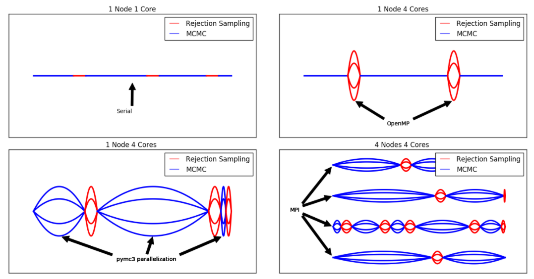
Our strategy for moving from a serial (top-left) to parallel implementation (bottom-right) is illustrated as follows. Lines represent nodes, webs represent processors.
Teleporting MCMC consists of two alternating sampling strategies; rejection sampling (red) and Markov chain Monte Carlo (blue). We distribute work across processors using:
- OpenMP (via Cython) for rejection sampling; and
- PyMC3's native support for multiple jobs for Hamiltonian MC.
We distribute work across nodes using MPI, specifically using mpi4py. Naive parallel code is available here, and our hybrid code (with test cases) is here. We also tested using OpenAcc and CUDA for GPU-based parallel rejection sampling, which can be seen here. Note that thorough testing is slightly less important for us because we evaluate our code via convergence metrics, which implicitly test correctness.
Synthetic Dataset
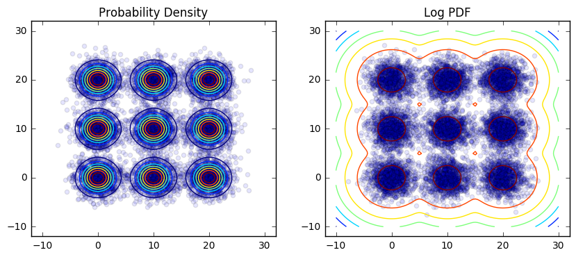
The model we chose to run our experiments against is the Gaussian mixture model. This problem is synthetic rather than real-world, but it has the advantage of being analytically tractable and easy to sample from, so we can easily evaluate a number of exact rather than approximate convergence metrics. We describe a major real-world application later on. Here are contour plots of the density of a 2D, 3x3 Gaussian mixture grid:
We implemented a parameterized class to generate Gaussian mixtures with varying dimensions, spacing, variance, and mode count:
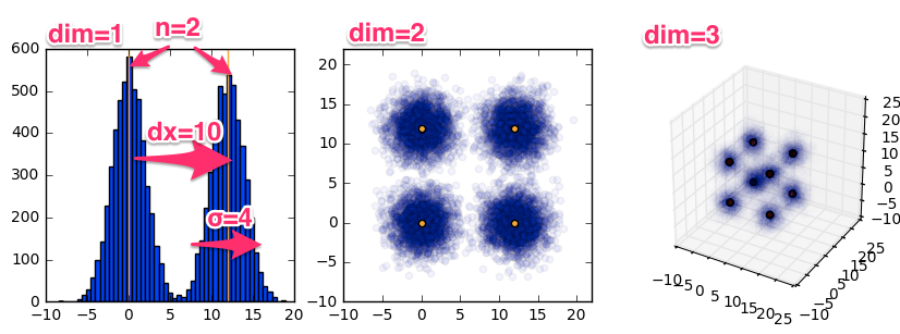
This gives us the flexibility to increase the multimodality and variance of our distribution while keeping the distribution tractable enough to accurately assess convergence.
Results
Which Method is Best?
The short answer? It depends (especially on dimensionality):
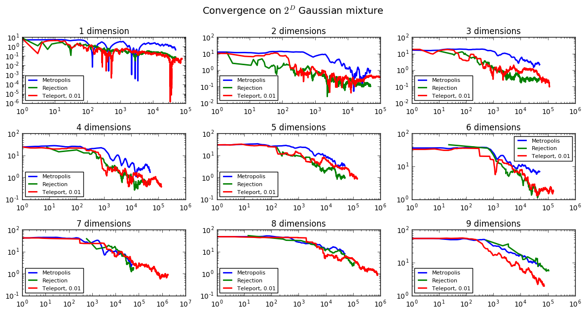
These results are for a grid with \(2^\text{number of dimensions}\) modes with a grid spacing of 25, and with each mode having a standard deviation of 4. Our teleporting algorithm is always at least as good as the best method, but it's not until we reach very high dimensions – 9, which corresponds to \(2^9=512\) modes – that it starts to outperform both the metropolis and rejection samplers.
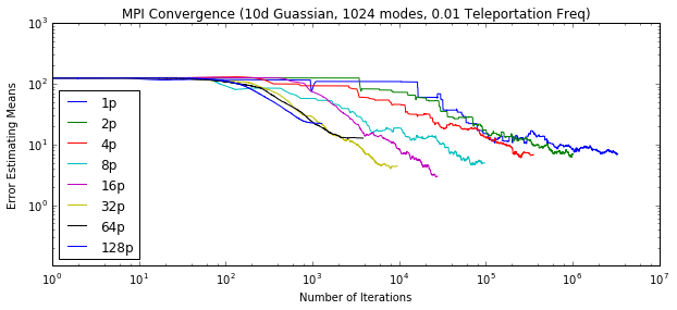
Those were plots for individual chains, but the main item of interest is how the results change with parallelism. Let's examine how the number of iterations until we reach a particular level of convergence (implementation details below) changes as we vary the number of parallel runs (note: these results are using our naive parallel implementation that does not parallelize the rejection sampling portion):
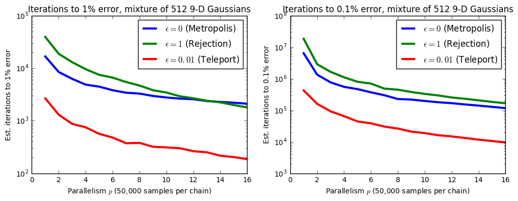
From these plots, the advantage of the teleporting sampler is clear, but what is also interesting is the difference in scaling behavior between the teleporting sampler and unaided Metropolis-Hastings (as well as how it varies with the tolerance). Because of the independence of its samples, rejection sampling is better able to exploit parallel resources even though its efficiency at 9 dimensions is only \(\approx 0.0008\) – less than one tenth of one percent. Metropolis isn't significantly helped by having more parallel chains because each chain is individually biased; they need to reach a minimum length before they fully contribute. Our teleporting sampler appears to get the best of both worlds; it only needs to rejection sample about every 100 iterations, but it's fairly unbiased, so it scales well.
When we need to reach a higher degree of precision, Metropolis-Hastings starts doing a little better compared to rejection sampling, even though the gap does start narrowing as we increase \(p\). Perhaps this is because the number of iterations per chain is several orders of magnitude higher, so each chain is closer to mixing.
Scaling vs. \(\epsilon\)
Independently of inter-method differences, we can also analyze intra-method speedups (moving back into linear from log space):
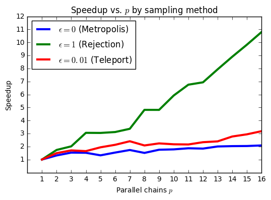
We included some of these results above in the background section because they felt useful not just as results but as characterizations of the methods themselves. Essentially, rejection sampling is serving as the gold standard: it produces uncorrelated samples, and so we should expect near-perfect speedup (almost equaling \(p\)). Metropolis produces highly correlated samples, so we should expect a much less significant speedup from parallelization. Finally, the teleportation method should be somewhere in between (which it is). Given a particular time vs. parallelism cost tradeoff, we should be able to choose a cost-optimal \(\epsilon\) for our sampler to reach a particular level of precision.
Why not perfect speedup for rejection sampling? As we explain below, these speedups are essentially measuring reduction in a standard deviation that depends both on the inefficiency of the sampler and on the underlying variance of the distribution. As we increase \(p\to\infty\), we expect the inefficiency of rejection sampling to go away completely since the samples are fully iid. However, there will still be an underlying variance inherent to the distribution, which will remain constant – essentially a minimum problem size.
We feel there may be interesting theoretical connections between ideas about overhead in parallel systems to variance in probabilistic ones.
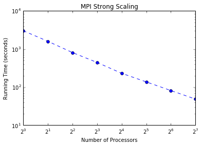
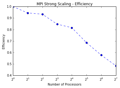
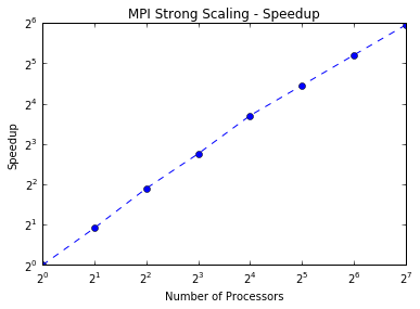
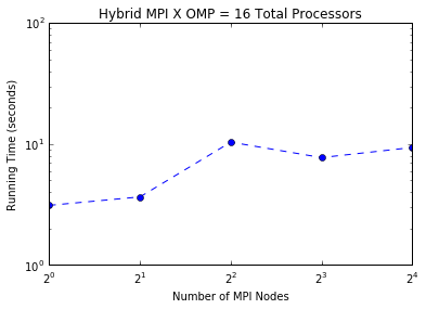
Speedups on Odyssey
First, using MPI (code here, we find we are able to run many, many parallel chains (up to 128) simultaneously. Our results show that for a fixed problem size we can achieve higher speedups by increasing the number of processors. The efficiency starts to drop with more processors, and thus MPI alone does not quite achieve strong scaling. However, for a fixed number of processors we can maintain a similiar efficiency for larger problem sizes.
These are just results for the naive parallel case using MPI. We pursued a hybrid approach to decrease the amount of MPI communication. We considered both OpenMP (code here) and OpenAcc (code here):
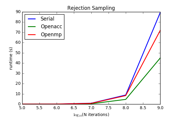
Although OpenACC is clearly somewhat faster, we settled on OpenMP for two reasons:
-
Generating random numbers within kernels is non-trivial. A naive approach would have each thread spin random numbers off a different seed. However, some random number generators fail to give independent sequences with different seeds which is particularly problematic when so many threads are involved. CUDA offers cuRAND to deal with randomness in a sophisticated manner and a bare bones implementation of rejection sampling using cuRAND is available in the repo. However with OpenACC the convention is to generate random numbers on the host and pass them to the device. This leads to increased communication overhead in terms of memory and time and impairs gains from harnessing the GPU.
-
Ease of integration with the Python framework (which housed the rest of our code).
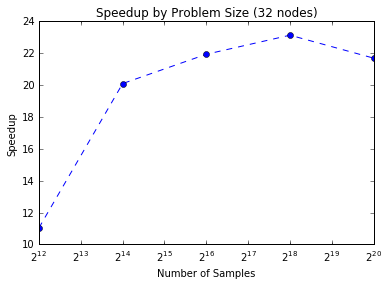
Below are our full hybrid results for speedup (final code here):
This plot is for 16 total processors/nodes which we allocate between MPI and OpenMP. The lowest runtime (the first dot) is when we allocate all of our processing power to OpenMP, suggesting that OpenMP is giving us the most bang for its buck on Odyssey. Clearly, given infinite parallel resources, we should use both OpenMP and MPI.
Convergence Details
Evaluating convergence is nontrivial because of the very same multimodality that makes our datasets difficult to sample. For our mixture of Gaussians, we take the following approach.
We begin with an array of samples and corresponding iteration indexes. The iteration index is not implied by the sample ordering because we may have discarded rejection samples in between final samples in our chain. If we have multiple parallel chains, we combine samples by mergesorting indexes.
We then take running averages across each sample dimension using a fast
implementation of cumsum (cumulative sum) and dividing by the index in the
array. This gives us an array of the cumulative sample average in each
dimension at each iteration.
We then subtract the overall mean of the mixture of Gaussians from the running sample averages and take the absolute value. This gives us absolute errors for each dimension at each iteration. Finally we sum across dimensions to obtain a total error by iteration. Although this took a while to explain, the code is quite compact.
From the central limit theorem, we know that the expected error of estimating a true mean from a mean across \(N\) samples should be
If we take this to log-log space, then this becomes:
This suggests that if we do a linear regression in log-log space to the error vs. the number of iterations, like this:
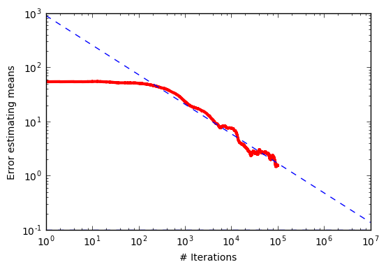
then we should obtain a slope of around -0.5 and an intercept that corresponds to the inherent variance of both the distribution and the sampling method. As expected, across sampling methods and independent trials, we see a clustering of slopes around -0.5:
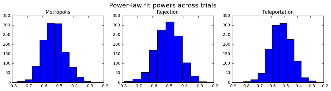
This suggests that we're following the central limit theorem, and we can somewhat justifiably take the linear intercept \(\log(\sigma)\) as a measure of how poorly we are converging. This quantity on its own is not that interpretable (although we could interpret it as the expected log error at 1 sample), but by comparing how it changes as we vary parallelism, we can generate speedup plots like the ones above and this one below:
However, we can also use our power law fit to simply extrapolate the time/iterations required to reach a specified convergence, which we do elsewhere. For more details, see this notebook.
Related Work
Other Methods
Other methods exist for sampling from multimodal distributions. A simple one is the idea of random restarts [11], where we start multiple chains at uniformly random points in state space, but weight the samples from each chain by the density at those random starting locations. This approach is similar in spirit to teleportation, except teleportation implicitly accounts for the downweighting by rejection sampling from the distribution itself, rather than uniformly. I believe for random restarts, also, the length of each chain is constant, whereas in teleportation it is random. Future work should investigate to what extent these methods are similar; given that rejection sampling is much less likely to place our chain in a region of near 0 probability, it is possible that random restarts will do a worse job of efficiently sampling the multimodal typical set than teleportation.
A more complex idea is parallel tempering, where we generate multiple replicas of an MCMC chain that each behave differently. In particular, each chain operates at a different "temperature," which determines the likelihood of sampling from a low probability region in the distribution of interest. Parallel tempering facilitates exploration by allowing each chain, operating at a different temperature, to exchange complete configurations. That is, chains operating at low temperatures can access regions more readily available to chains running at high temperatures. This has been found to converge much faster than vanilla MCMC, but tuning temperature values for each chain can be difficult. Moreover, the algorithm may not scale well, because the procedure for swapping states is sensitive to the overlap in search between those two states. It would be interesting to compare this with our method, or even to investigate combining them.
We almost neglected to mention Hamiltonian Monte Carlo [12] because it is so ubiquitous; it is a major improvement on top of normal Metropolis-Hastings that is able to sample high-dimensional distributions much more efficiently by utilizing local gradient information about the probability distribution. Although HMC is efficient at overcoming "low energy barriers" in partially multimodal problems, where modes are separate but still connected by regions of nonzero probability, HMC suffers from the same issues as Metropolis-Hastings in sampling truly multimodal distributions (which we might expect for any gradient-based method faced with nonconvexity). Hamiltonian Monte Carlo should not be seen as a competitor to our method; for ease of implementation, we implemented our teleportation algorithm on top of Metropolis-Hastings, but for future work, we would implement HMC with teleportation to make the local sampling steps more efficient.
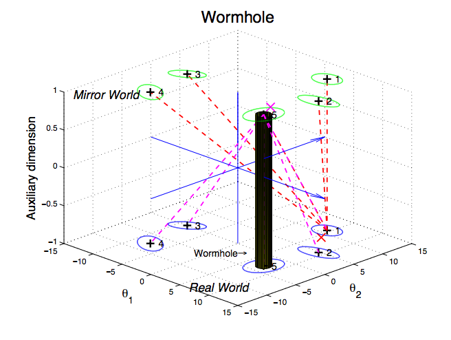
Finally, we should mention other attempts to improve on HMC. Wormhole Hamiltonian Monte Carlo [4] adds auxiliary dimensions to the normal problem of sampling to create a "mirror world." Within this augmented mirror world, normally disconnected modes become close in proximity in the auxiliary dimension. Modes are connected in a network. For simple problems, the modes can specified beforehand, but in general Wormhole HMC attempts to discover them during normal HMC with random restarts. This complicates the implementation of the algorithm and still produces biased results if all modes are not discovered. However, after they are, Wormhole HMC samples extremely efficiently.
Application: Noisy Sensors
One real-world application to which we can directly apply our method is sensor localization, which is discussed by both [4] and [5].
The setup for this problem is as follows. Assume we have a collection of \(N\) sensors with 2D or 3D locations \(\vec{x}_k\) which noisily attempt to communicate with each other. For any pair of sensors \(i\) and \(j\), there is an exponentially decreasing probability they can communicate at all, indicated by
Assuming \(Z_{ij} = 1\), i.e. that they do manage to communicate, they transmit a noisy measurement of their distance
where \(R\) and \(\sigma\) are known sensor parameters. The total probability of observing our data \(Y\) and \(Z\) given our locations \(\vec{x}\) is just the product of all of these terms for each \(i, j\) pair.
In general we are interested in the reverse problem; we have the measurement data but do not know the sensor locations. However, assuming a uniform prior on the sensor locations, the probability of the locations given the data is proportional to the probability of the data given the locations. For both MCMC and rejection sampling, this is enough; we do not need to know the normalizing constant of our distribution, just its relative density at each location.
In general (as you might imagine), the resulting posterior distributions of sensor locations given measurement data are often multimodal, sometimes with many different modes for each sensor. In the case below, which is for \(N=8\) on a 2D grid (with three extra sensors with known locations, to resolve mirror symmetry ambiguities), we have a 16-dimensional posterior distribution of the \(x,y\) locations of each sensor, whose marginals are projected onto a 2D plane (with true locations represented as circles):

As you can see, there is true multimodality to this real-world problem, with multiple valid hypotheses for the locations of many sensors, which, as [4] shows, many state of the art MCMC methods fail to adequately capture. Given additional time, it would be straightforward to apply our method to this problem, and we believe it could be competitive with the algorithms presented in [4] and [5], especially if \(\epsilon\) is tuned to optimize parallel resources.
Connections to PageRank
As a brief aside, our method has some interesting connections to PageRank [9], an enormously successful MCMC algorithm that Google used to determine a sensical popularity-based order of pages on the web. It essentially operates by doing a random walk over the entire web and ranking pages based on how often they are visited.
The issue is that there are disconnected subgraphs in the web (which are kind of like a discrete analogue to multimodality or non-convexity in a probability distribution), which makes the random walk impossible. This means that the standard method for running MCMC over discrete graphs, the power iteration (which essentially just extracts eigenvalues corresponding to the final ranks via a series of matrix multiplications – almost a classic parallel algorithm), doesn't work. The transition matrix is singular. PageRank resolves this by adding a small "teleportation" term which essentially adds a chance of jumping to an entirely random page at any point in the random walk. Schematically, this can be illustrated as follows:
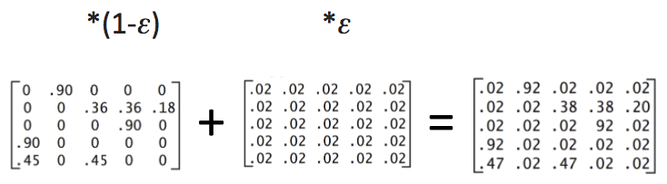
Or in graph form:
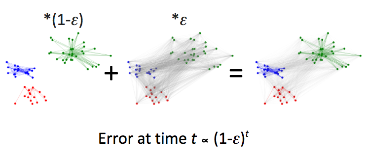
The resulting matrix is no longer singular, although its condition number will be high and convergence will be slow if \(\epsilon\) is too small (see [8] and [7]). If \(\epsilon\) is too high, then the distribution becomes uniform and the distinction between pages blurs. But there is a happy medium where the problem is well-conditioned, converges quickly, and the results provide a meaningful ranking of pages.
This simple discrete example has close conceptual connections to our approach on sampling. Instead of a discrete but disconnected graph, we have a multimodal probability distribution, and again we speed up the inherent convergence properties of our MCMC algorithm by adding a small probability of teleportation everywhere. Unlike PageRank, increasing \(\epsilon\) does not change the distribution, because our teleportation uses rejection samples from the probability distribution itself, but it does come at the cost of a computationally inefficient process to obtain the next rejection sample. This problem is of interest in this class in particular because our tradeoff also involves a change in the parallel scaling behavior of the algorithm.
Conclusions
Checking the Boxes
To summarize, in this project we have:
- Devised a novel sampling method for intractable multimodal distributions, which arise in problems like sensor localization and topic modeling.
- Investigated the parallel scaling properties inherent to both the algorithm and the problem, with particular focus on the sampling efficiency vs. parallel scaling tradeoffs.
- Implemented both naive and hybrid parallel versions of our algorithm using MPI, OpenMP, OpenAcc, and multi-process parallelelism, demonstrating strong scaling along the way.
Discussion and Future Work
One main thing we would attempt to determine next would be the (cost or time) optimal \(\epsilon\) for a given distribution and set of parallel resources. We have demonstrated that, at the very least, neither \(\epsilon=0\) nor \(\epsilon=1\) is optimal for a high dimensional Gaussian mixture model, but we have not found the best value.
Another complexity that should be analyzed is how much our method of parallelizing rejection sampling (within each MPI node) affects this optimal \(\epsilon\). Because of this strong coupling between parallel scaling and \(\epsilon\), improving the parallelism of our algorithm could potentially mean that we must choose a higher value if we want to reach a specified convergence threshold in a cost-optimal manner.
Finally, we would like to shore up our theoretical analysis of the relationship between the variance of the distribution and the scaling properties of samplers. In general, we think there is value in trying to bridge the conceptual gaps between parallel computing and statistics, optimization, and numerical methods, which are subjects we have all been studying "in parallel" in the CSE program. We hope that by sampling all of these academic modes together, with plenty of jumping back and forth, we can ultimately converge on better solutions to the big science problems that motivate them all.
References
- Solonen, Antti, et al. "Efficient MCMC for climate model parameter estimation: parallel adaptive chains and early rejection." Bayesian Analysis 7.3 (2012): 715-736.
- Geweke, John, and Charles Whiteman. "Bayesian forecasting." Handbook of economic forecasting 1 (2006): 3-80.
- Ceperley, D. M. "Metropolis methods for quantum Monte Carlo simulations." AIP Conference Proceedings. Ed. James E. Gubernatis. Vol. 690. No. 1. AIP, 2003.
- Lan, Shiwei, Jeffrey Streets, and Babak Shahbaba. "Wormhole Hamiltonian Monte Carlo." Proceedings of the AAAI Conference on Artificial Intelligence. AAAI Conference on Artificial Intelligence. Vol. 2014. NIH Public Access, 2014.
- Ahn, Sungjin, Yutian Chen, and Max Welling. "Distributed and Adaptive Darting Monte Carlo through Regenerations." AISTATS. 2013.
- Roberts, Margaret, Brandon Stewart, and Dustin Tingley. "Navigating the local modes of big data: The case of topic models." 2015.
- Haveliwala, Taher, and Sepandar Kamvar. The second eigenvalue of the Google matrix. Stanford, 2003.
- Backåker, Fredrik. The Google Markov Chain: convergence speed and eigenvalues. Diss. Master Thesis, Uppsala University, Sweden, 2012.
- Page, Lawrence, et al. The PageRank citation ranking: Bringing order to the web. Stanford InfoLab, 1999.
- Radford M. Neal (1996). "Sampling from multimodal distributions using tempered transitions". Statistics and Computing. 6 (4): 353–366.
- Barrett, Leon, and Aleksandr Simma. "MCMC With Disconnected State Spaces." (2005).
- Neal, Radford M. "MCMC using Hamiltonian dynamics." Handbook of Markov Chain Monte Carlo 2 (2011): 113-162.